When you use ChatGPT, stream Netflix recommendations, or see personalized ads, sophisticated machine learning optimizers work behind the scenes. These optimization algorithms are the mathematical engines that enable AI models to learn from data and improve prediction accuracy. In this comprehensive guide, we’ll explore how optimizers work, compare popular algorithms, and examine their real-world applications.
What Are Machine Learning Optimizers?
Machine learning optimizers are algorithmic components responsible for adjusting model parameters (weights and biases) to minimize prediction errors during neural network training. Think of them as GPS systems for AI models, constantly recalculating the best route toward optimal performance.
The Mathematical Foundation of Optimization
The gradient descent optimization process centers around this fundamental equation:
θ = θ - α · ∇J(θ)
Where:
- θ represents model parameters
- α is the learning rate (step size)
- ∇J(θ) is the gradient of the loss function
This equation shows how deep learning models iteratively improve by moving parameters in directions that reduce overall error.
Gradient Descent: The Foundation of Neural Network Training
Gradient descent algorithm serves as the cornerstone of machine learning optimization. This first-order method works through:
- Computing gradients: Calculating how the loss function changes with respect to each parameter
- Taking optimization steps: Moving parameters in the direction of steepest descent
- Iterative improvement: Repeating until convergence to optimal solutions
Limitations of Standard Gradient Descent
Traditional gradient descent faces several challenges:
- Processes entire datasets before each parameter update
- Computationally expensive for big data machine learning
- Can get trapped in local minima
- Slow convergence on large datasets
Stochastic Gradient Descent (SGD): Revolutionizing AI Training
Stochastic Gradient Descent transformed neural network optimization by introducing efficiency and scalability:
Key Advantages of SGD Algorithm
- Faster convergence: Updates parameters using mini-batches instead of full datasets
- Memory efficient: Processes smaller data chunks for scalable machine learning
- Noise benefits: Random sampling helps escape local minima
- Online learning capability: Adapts to new data in real-time
Real-World SGD Applications
- Computer vision: Training convolutional neural networks on millions of images
- Natural language processing: Processing vast text corpora for large language models
- Recommendation systems: Continuously updating user preferences for personalized content
- Autonomous vehicles: Real-time learning for perception systems
Advanced Machine Learning Optimizers
Momentum-Based Optimization Methods
Momentum optimization enhances gradient descent by incorporating historical gradient information:
- Smoother convergence: Reduces oscillations in irrelevant directions
- Accelerated training: Builds velocity in consistent gradient directions
- Better navigation: Helps traverse complex loss landscapes
Application Example: Training deep neural networks for medical image analysis, where momentum helps navigate loss landscapes with multiple local minima.
Adaptive Learning Rate Optimizers
AdaGrad Optimizer
AdaGrad algorithm adapts learning rates individually for each parameter:
- Sparse data optimization: Provides larger updates to infrequent features
- Automatic parameter scaling: Adjusts based on historical gradient magnitudes
- Search engine optimization: Ideal for keyword relevance where rare terms are significant
Limitation: Learning rates may decrease too rapidly, causing premature convergence.
RMSprop Algorithm
RMSprop optimizer addresses AdaGrad’s limitations:
- Exponential gradient averaging: Uses moving average of squared gradients
- Consistent learning rates: Prevents premature convergence in deep learning training
- Stable optimization: Maintains effectiveness throughout the training process
Adam Optimizer: The Gold Standard
Adam optimization algorithm (Adaptive Moment Estimation) combines momentum and adaptive learning rates, making it the most popular choice for modern machine learning:
Adam Optimizer Features
- Dual moment estimation: Tracks both mean and variance of gradients
- Bias correction: Adjusts for initialization bias in early training
- Robust performance: Works effectively across diverse AI model architectures
- Minimal hyperparameter tuning: Requires fewer manual adjustments
Industry Applications of Adam Optimizer
- Computer vision models: Training state-of-the-art image classification algorithms
- Speech recognition: Optimizing transformer architectures for voice assistants
- Autonomous driving: Training perception systems for real-time decision making
- Financial AI: Optimizing algorithmic trading models and fraud detection systems
Common Optimization Challenges in Deep Learning
Vanishing and Exploding Gradients
Deep neural network training faces gradient stability issues:
Gradient Problems
- Vanishing gradients: Information loss in deeper network layers
- Exploding gradients: Unstable, divergent training behavior
Optimization Solutions
- Gradient clipping: Limiting maximum gradient magnitude for stability
- Weight initialization: Using Xavier or He initialization techniques
- Batch normalization: Normalizing inputs to each layer for stable training
Learning Rate Scheduling Strategies
Dynamic learning rate adjustment improves neural network convergence:
Common Scheduling Techniques
- Step decay: Reducing learning rate at predetermined intervals
- Exponential decay: Gradual, continuous learning rate reduction
- Cosine annealing: Smooth, periodic learning rate adjustments
- Warm restarts: Periodic learning rate resets for better exploration
Real-world Example: Training large language models like GPT where initial high learning rates enable rapid progress, then gradual reduction allows fine-tuning.
Regularization in Optimization
Modern optimizers integrate regularization techniques to prevent overfitting:
- L1 regularization: Encourages sparse, interpretable models
- L2 regularization: Prevents excessive parameter magnitudes
- Dropout optimization: Randomly deactivating neurons during training
Machine Learning Optimization Best Practices
Batch Size Optimization
Choosing appropriate training batch sizes involves important trade-offs:
Small Batches (32-128)
- More frequent parameter updates
- Higher gradient noise for exploration
- Better for memory-constrained environments
Large Batches (512-1024+)
- More stable gradient estimates
- Better GPU parallelization efficiency
- Requires more computational memory
Industry Example: GPT model training uses large batch sizes for stability, while mobile AI applications use smaller batches for memory constraints.
Computational Efficiency in AI Training
Modern optimization frameworks balance effectiveness with efficiency:
- Mixed-precision training: Using 16-bit floats to reduce memory usage
- Gradient accumulation: Simulating large batches with limited memory
- Distributed optimization: Scaling across multiple GPUs or cloud instances
- Model parallelism: Splitting large models across multiple devices
Future of Machine Learning Optimization
Emerging Optimization Trends
The AI optimization landscape continues evolving rapidly:
Current Research Areas
- Second-order optimization methods: Using curvature information for faster convergence
- Meta-learning optimizers: Algorithms that learn optimal optimization strategies
- AutoML optimization: Automatically tuning hyperparameters for optimal performance
- Quantum-inspired optimizers: Leveraging quantum computing principles
Industry Impact and Applications
- Edge AI computing: Developing lightweight optimizers for mobile and IoT devices
- Federated learning: Optimizing across distributed, privacy-preserving data sources
- Neural architecture search: Automatically designing optimal deep learning architectures
- Green AI: Developing energy-efficient optimization for sustainable machine learning
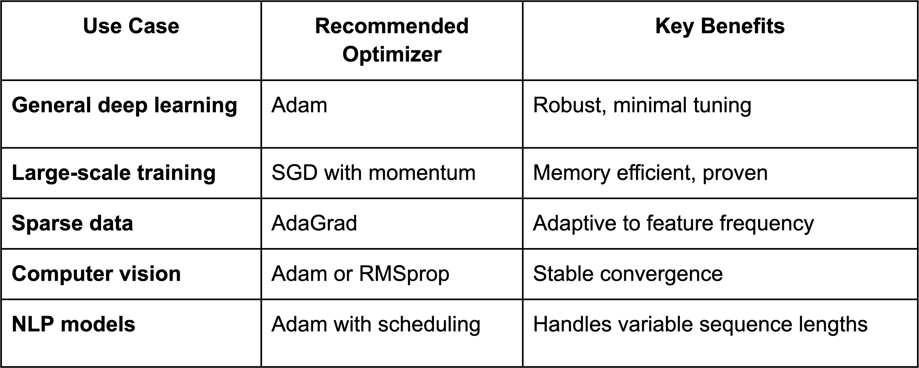
Choosing the Right Optimizer for Your Project