Every time you get accurate Netflix recommendations, your smartphone recognizes your voice, or an autonomous car safely navigates traffic, loss functions in machine learning are working behind the scenes. These mathematical powerhouses serve as the compass that guides AI models toward making better predictions by measuring the gap between what a model predicts and what actually happens.
What Are Loss Functions in Machine Learning?
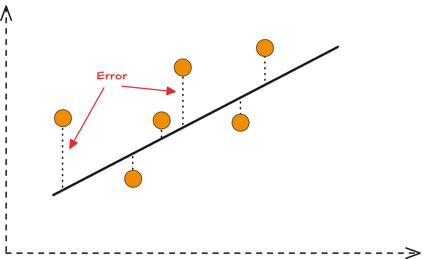
Loss functions are mathematical formulas that quantify how far off a machine learning model’s predictions are from the actual target values. Think of them as scorekeepers in the world of AI—they tell optimization algorithms exactly how wrong the model is and in which direction to improve.
The Mathematical Foundation of Loss Functions
At its core, a loss function transforms the abstract concept of “model accuracy” into concrete numbers that computers can work with. The fundamental goal is simple: minimize the loss to maximize model performance.
Key Components:
- Individual loss: Error calculation for single predictions
- Cost function: Average loss across entire training datasets
- Gradient generation: Directional guidance for parameter updates
- Optimization feedback: Critical input for learning algorithms
This mathematical framework enables neural networks and other machine learning algorithms to learn systematically from data.
Why Loss Functions Matter in Deep Learning
Loss functions serve as the critical bridge between model predictions and the optimization process. During neural network training, models make predictions, loss functions evaluate accuracy, and this evaluation generates gradients that guide parameter adjustments.
The Training Feedback Loop
The iterative machine learning training process relies on this essential feedback mechanism:
- Model prediction: Neural network generates output
- Loss calculation: Function measures prediction accuracy
- Gradient computation: Determines parameter adjustment direction
- Weight updates: Optimizer improves model parameters
- Repeat: Process continues until convergence
Without loss functions, AI models would lack the directional guidance necessary for systematic improvement.
Regression Loss Functions: Predicting Continuous Values
Mean Squared Error (MSE): The Foundation
Mean Squared Error (MSE) is the most fundamental regression loss function for predicting continuous values like house prices, stock prices, or temperature forecasts.
MSE Formula:
MSE = (1/n) × Σ(actual - predicted)²
MSE Advantages and Applications
- Gradient-friendly: Smooth derivatives enable stable optimization
- Penalizes large errors: Squared terms emphasize significant mistakes
- Computationally efficient: Simple calculation for large datasets
- Standard benchmark: Widely used baseline for regression tasks
Real-World MSE Applications:
- Financial forecasting: Predicting stock prices and market trends
- Weather prediction: Temperature and precipitation forecasting
- Sales forecasting: Revenue and demand prediction models
- Medical diagnosis: Continuous biomarker prediction
Mean Absolute Error (MAE): Robust to Outliers
Mean Absolute Error (MAE) provides an alternative regression loss function that’s more robust to outliers than MSE.
MAE Benefits:
- Outlier resistance: Linear treatment of all errors
- Interpretable: Direct average of absolute differences
- Balanced sensitivity: Equal weight to all prediction errors
- Robust optimization: Stable gradients for diverse datasets
Industry Applications:
- Supply chain optimization: Inventory and logistics forecasting
- Energy management: Power consumption prediction
- Healthcare analytics: Patient outcome forecasting with noisy data
Huber Loss: Best of Both Worlds
Huber loss combines MSE and MAE advantages, providing a hybrid approach for robust machine learning:
- Small errors: Behaves like MSE for precise optimization
- Large errors: Transitions to MAE behavior for outlier resistance
- Adaptive sensitivity: Adjusts behavior based on error magnitude
- Stable training: Maintains gradient flow in deep neural networks
Classification Loss Functions: Predicting Categories
Binary Cross-Entropy Loss: Two-Class Problems
Binary cross-entropy loss is the gold standard for binary classification tasks like spam detection, medical diagnosis, or fraud detection.
Mathematical Formula:
BCE = -[y×log(p) + (1-y)×log(1-p)]
Binary Cross-Entropy Applications
Key Advantages:
- Probability calibration: Outputs well-calibrated probabilities
- Strong gradients: Provides clear optimization signals
- Sigmoid compatibility: Works perfectly with sigmoid activation
- Interpretable outputs: Direct probability interpretation
Real-World Binary Classification:
- Email security: Spam vs. legitimate email detection
- Medical screening: Disease presence/absence prediction
- Credit scoring: Loan approval/rejection systems
- Fraud detection: Transaction legitimacy assessment
Categorical Cross-Entropy: Multi-Class Classification
Categorical cross-entropy loss extends binary classification to multiple classes, essential for multi-class classification problems.
Use Cases and Benefits:
- Image recognition: Classifying objects into multiple categories
- Natural language processing: Sentiment analysis with multiple emotions
- Recommendation systems: Predicting user preferences across categories
- Computer vision: Medical image classification into multiple conditions
Industry Applications:
- E-commerce: Product categorization and recommendation
- Social media: Content classification and moderation
- Autonomous vehicles: Object detection and classification
- Healthcare: Multi-disease diagnosis from medical imaging
Hinge Loss: Maximum Margin Classification
Hinge loss focuses on creating robust decision boundaries, originally popularized by Support Vector Machines but now used in neural networks.
Hinge Loss Benefits:
- Margin maximization: Creates robust decision boundaries
- Sparsity promotion: Focuses on difficult examples near boundaries
- Computational efficiency: Simple calculation for large datasets
- Robust classification: Handles noisy data effectively
Advanced Loss Function Concepts
Regularization in Loss Functions
Regularized loss functions prevent overfitting by adding penalty terms that discourage model complexity:
L1 Regularization (Lasso)
- Feature selection: Promotes sparse models
- Automatic variable selection: Reduces irrelevant features
- Interpretability: Creates simpler, more understandable models
L2 Regularization (Ridge)
- Weight decay: Prevents extremely large parameters
- Smooth solutions: Encourages balanced feature usage
- Numerical stability: Improves optimization convergence
Regularized Loss Formula:
L_regularized = L_original + λ × R(parameters)
Where λ controls regularization strength and R represents the penalty term.
Choosing the Right Loss Function: Decision Guide
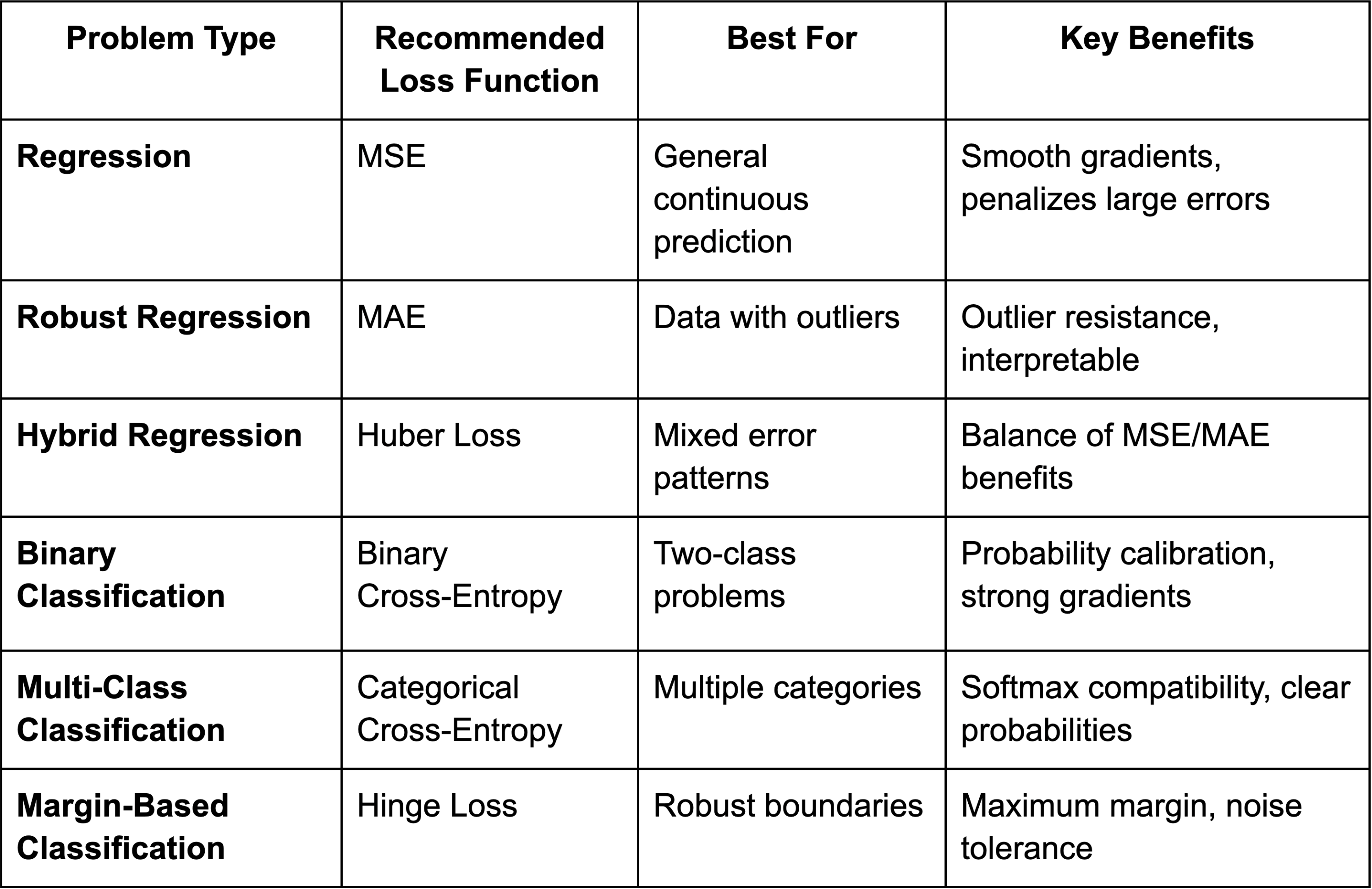
Data-Driven Selection Criteria
Dataset Characteristics:
- Outlier presence: Choose MAE or Huber for robust handling
- Class imbalance: Consider weighted loss functions
- Noise levels: Robust losses for noisy data
- Dataset size: Simple losses for large-scale training
Model Requirements:
- Probability outputs: Cross-entropy for calibrated probabilities
- Feature selection: L1-regularized losses for sparsity
- Computational constraints: Simple losses for efficiency
- Interpretability needs: MAE for direct error interpretation
Loss Functions in Modern Deep Learning
Custom Loss Functions for Specialized Tasks
Modern AI applications often require custom loss functions tailored to specific objectives:
Domain-Specific Examples:
- Computer vision: Perceptual loss for image generation quality
- Recommendation systems: Ranking loss for personalized suggestions
- Generative AI: Adversarial loss for realistic content creation
- Medical AI: Focal loss for rare disease detection
Loss Landscape Optimization
Loss landscapes—how loss values change across parameter space—critically impact neural network training:
Landscape Properties:
- Smoothness: Enables stable gradient descent
- Convexity: Guarantees global optima (rare in deep learning)
- Local minima: Multiple optimal solutions in complex models
- Saddle points: Training challenges in high-dimensional spaces
Numerical Stability in Practice
Production loss functions must handle numerical edge cases:
Implementation Considerations:
- Logarithm stability: Clip inputs to prevent infinite values
- Exponential overflow: Use numerical tricks for large values
- Gradient clipping: Prevent exploding gradients
- Mixed-precision training: Maintain accuracy with efficiency
Monitoring Loss Functions During Training
Loss Curve Analysis
Training loss patterns reveal critical insights about model performance:
Healthy Training Patterns:
- Decreasing loss: Consistent improvement over epochs
- Convergence: Loss stabilization at optimal values
- Smooth curves: Stable optimization without oscillations
Warning Signs:
- Increasing loss: Potential overfitting or learning rate issues
- Oscillating loss: Unstable optimization requiring adjustment
- Plateauing loss: Need for learning rate decay or architecture changes
Validation Loss Monitoring
Validation loss tracking prevents overfitting and ensures generalization:
- Early stopping: Halt training when validation loss increases
- Hyperparameter tuning: Optimize based on validation performance
- Model selection: Choose architectures with best validation scores
- Regularization adjustment: Balance training and validation performance
Emerging Trends in Loss Function Design
Adaptive and Learned Loss Functions
Next-generation loss functions adapt to data characteristics automatically:
Research Directions:
- Meta-learning losses: Automatically discover optimal functions
- Curriculum learning: Gradually increase loss complexity
- Dynamic weighting: Adjust loss components during training
- Adversarial losses: Competitive training for improved robustness
Multi-Objective Optimization
Modern applications often require balancing multiple objectives:
Multi-Objective Approaches:
- Weighted combinations: Balance accuracy, fairness, and efficiency
- Pareto optimization: Find optimal trade-offs between objectives
- Hierarchical losses: Priority-based objective optimization
- Constraint incorporation: Hard constraints within loss functions
Best Practices for Loss Function Implementation
Production Deployment Considerations
Real-world loss function deployment requires careful engineering:
Performance Optimization:
- Vectorized computation: Leverage GPU acceleration
- Batch processing: Efficient large-scale calculation
- Memory management: Optimize for large dataset training
- Gradient checkpointing: Balance memory and computation
Monitoring and Debugging:
- Loss visualization: Track training progress effectively
- Gradient analysis: Detect vanishing/exploding gradients
- Statistical monitoring: Detect distribution shifts in production
- A/B testing: Compare loss function performance empirically
Future of Loss Functions in AI
Quantum and Neuromorphic Computing
Emerging computing paradigms will influence loss function design:
- Quantum loss functions: Leverage quantum superposition for optimization
- Neuromorphic losses: Mimic biological learning mechanisms
- Energy-efficient losses: Optimize for low-power edge computing
- Federated losses: Privacy-preserving distributed optimization
Integration with Human Feedback
Human-in-the-loop learning incorporates human preferences directly into loss functions:
- Reinforcement learning from human feedback (RLHF): Used in ChatGPT and similar models
- Preference learning: Optimize based on human choice data
- Interactive optimization: Real-time loss adjustment based on feedback
- Ethical constraints: Incorporate fairness and safety into loss design
Conclusion: Mastering Loss Functions for Better AI
Loss functions are the mathematical engines that transform human objectives into algorithmic optimization targets. From fundamental MSE regression to sophisticated multi-objective optimization, these functions determine how effectively AI models learn from data.
Understanding loss function selection, implementation, and monitoring is crucial for developing robust machine learning systems. Whether you’re building computer vision models, natural language processing systems, or recommendation engines, choosing the right loss function significantly impacts model performance and business outcomes.